
Detecting Pavement Distress with Deep Learning for Computer Vision
Some views and findings about this relatively new tool in the pavement engineer and road asset engineer's arsenal

Ever since I have been involved in road rehabilitation design and road asset management, knowing the exact location and extent of pavement distress has been the holy grail of pavement condition information.
I can recall, in the early 1990’s, walking with a clipboard up and down on-and-off ramps to record distresses on the busy M2 Motorway in Johannesburg. I recall doing the same a decade later in Johor Bahru at the southern end of Malaysia, and then spending weeks trying to piece together strip-maps showing distress locations in a way that would enable me to optimally decide on treatment types and locations.
The restriction of having to physically inspect the road, with the safety risks associated with field inspections1, meant that a complete and precise map of distress type and location remained a goal out of reach. That is why I am excited about the possibilities of the new emerging Deep Learning for computer vision technology which uses Artificial Intelligence to detect distresses and road assets from videos.
Now, at last, I feel we are moving toward readily accessible and cost effective mapping of distresses both for project-and-network level needs.
Through our Juno Intelligence (JI) tool-set, Lonrix is fast becoming a leader in providing cost-effective inferencing of distress and road assets. This technology now means that an extensive survey of distresses can be obtained with an equipment cost for a GoPro camera costing little over $1,000. In my view, this makes an inexpensive video survey one of the most cost effective network survey types available2.
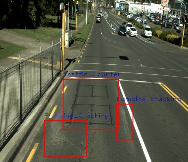
From a pavement engineering perspective, one of the key advantages of this technology is that it allows us to not only estimate the quantum of any specific distress on a road segment, but also the exact location of the distresses. This means we can now move toward a rational determination of whether the distresses are isolated or indicative of systemic distress.
At present, one of our key drivers in this area is to rationally and honestly assess the quality of the data we get from our inferencing system.
In my previous post I mentioned how our team was using Machine Learning to reverse engineer the factors that drive decisions related to the assignment of treatments in field validation of a Forward Works Programme. I showed that Alligator Cracking was perhaps the most important determinant influencing whether or not a treatment was assigned to a segment.
For a while now, I have been working with the JI team to try and assess the accuracy and fitness-for-purpose of the distresses assigned by our JI-system. Given the importance of Alligator cracking, I was particularly interested to review how well Alligator cracking data from our JI computer vision technology compared with data recorded with traditional field surveys.
One data set pertains to a large city in New Zealand for which we had visual inspections performed in accordance with the NZ RAMM visual inspection system. With this set, we summed - for each distress type - the distress lengths obtained from our JI-system on each inspection length on which distresses were recorded with the RAMM rating system.
Unfortunately, there are several limitations that make a direct comparison of distress areas or lengths with these two approaches impractical. A key constraint here is that the JI-system does not record exactly the same distress types as is prescribed in the RAMM rating system. For this reason, I did not attempt a direct correlation of distress quantities, but rather focused on the ranking of segments based on estimated alligator cracking.
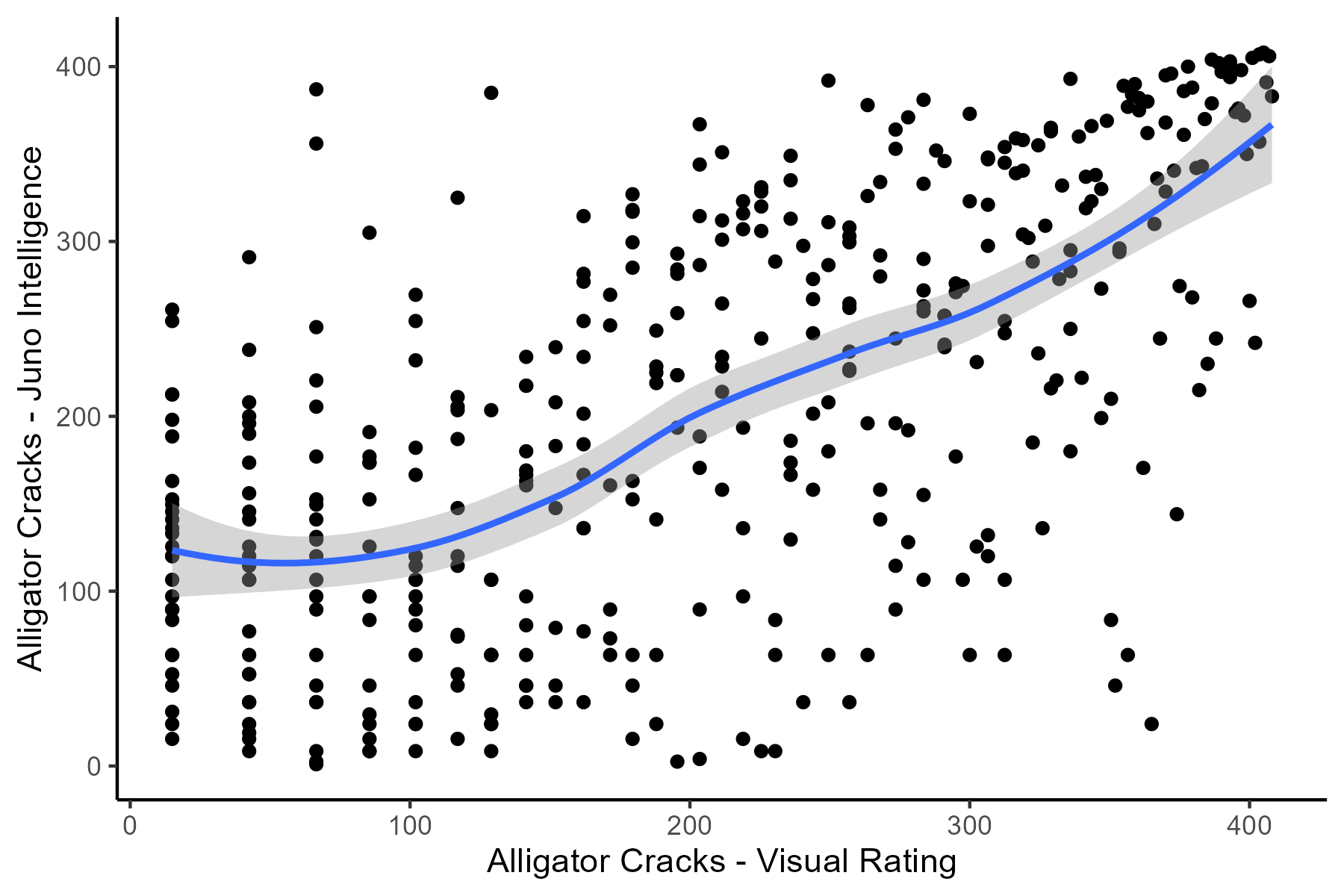
The data set at my disposal had 4,219 inspection segments. When I perform a Spearman Rank correlation between the rankings based on Alligator cracking with the two systems (visual rating vs video-inferencing), I get a Spearman Correlation Coefficient of 0.632 with a Spearman P-value close to zero indicating a significant correlation between the two data sets.
There are many outliers, however, as the ranking comparison plot below shows. This plot shows the ranking order for each segment on which alligator cracking was recorded by either system. The blue line shows a trend with a 95th percentile confidence band.
Another way to compare these two different ways of quantifying distress is to investigate the number of segments that match when we consider only say the 400 segments with the highest quantity of distress identified with the two methods (this comprises roughly the worst 10%). The result looks as follows:
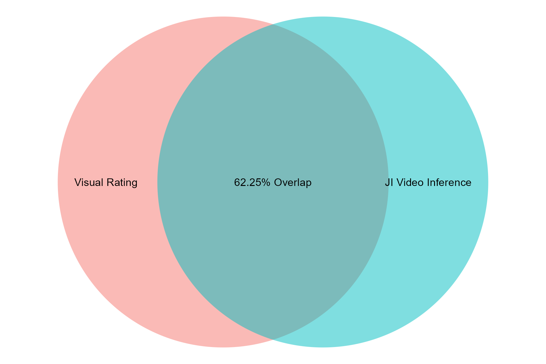
In my view, this is a good outcome given the differences in the way distress is recorded, the exact details of what is being recorded etc. At this stage, we are keeping in mind that the Visual Rating cannot be taken as the ground truth. Putting aside the known problems with subjective assessments of distress, there is also the grey area between longitudinal cracking and crocodile cracking - when, exactly, does a longitudinal crack become an alligator crack?
Having said that, at Lonrix we have made a principled decision to under-promise and over-deliver. We are well aware that there is room for improvement in this technology, and we are determined to push forward with a view towards excellence.
Tragically, one of my team mates during my time working in Malaysia in 2000/2001 was later killed when a vehicle ran into a construction/inspection zone where he was working.
If you are doing inferencing to detect distresses and/or road assets using video data, then of course there are additional costs involved. However, I believe these costs compare well with the costs of other survey types. Plus, you now have a video of your network available that you can return to repeatedly for validation purposes.